Learn RAG by Actually Seeing How It Works

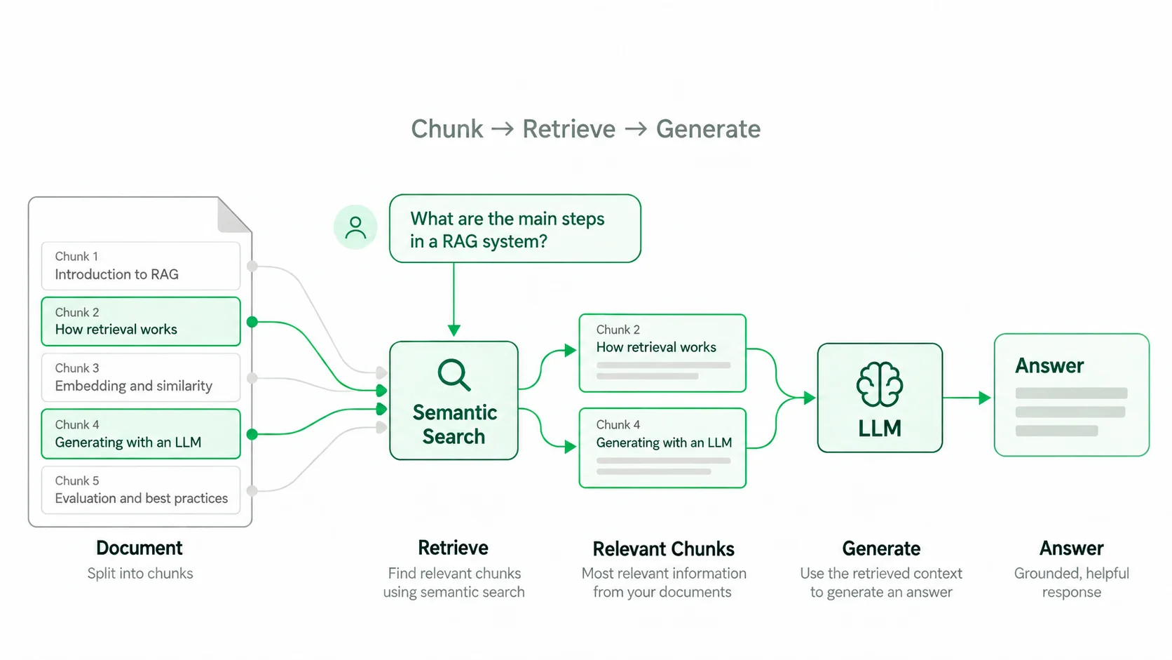
Retrieval-Augmented Generation(RAG) sounds complicated when you first encounter terms like embeddings, vector databases, semantic search, cosine similarity, chunking, and retrieval scores.

But the basic idea is surprisingly simple.

In this tutorial, we are going to understand RAG from the ground up. More importantly, instead of only talking about the theory, we will use Predictable Dialogs to actually see a RAG pipeline working.

The goal is not initially to build RAG yourself. The first goal is to understand exactly what is happening.

Once you understand the pipeline, it becomes much easier to explore vector databases, embedding models, rerankers, hybrid search, and eventually build the individual components yourself.

RAG starts with search

There are two major steps:

1. Retrieval: Find information that is relevant to the user's question.
2. Generation: Give that information to an LLM and ask it to generate an answer.

Before understanding RAG, we need to understand retrieval. One of the most common ways to retrieve information in RAG is semantic search.

What is semantic search?

Imagine that you have uploaded a document containing hundreds of pages. A user asks:

What is our cancellation policy?

Somewhere inside those pages might be a paragraph explaining cancellations. The first problem is how to find the right paragraph.

Traditional search often works by matching words. A keyword search for “cancellation policy” might look for passages containing “cancellation” and “policy.”

Semantic search works differently. Instead of asking “Which passages contain these words?” it tries to ask “Which passages have a similar meaning?”

A document might say:

Customers may terminate their subscription within 30 days.

The question might say:

Can I cancel my subscription?

The wording is different, but the meaning is closely related. Semantic search is designed to find these relationships. To do that, we use embeddings.

What is an embedding?

An embedding is a numerical representation of information. Suppose we have the sentence:

Customers can cancel their subscription within 30 days.

An embedding model converts that sentence into a vector containing many numbers. Conceptually, it might look like this:

[0.23, -0.17, 0.91, 0.04, -0.52, ...]

Wait, You do not need to understand the above, to understand RAG.

You just need to know that Real embedding vectors can contain hundreds or thousands of dimensions.

The dimensions are learned during training.

What matters is that the resulting vectors let us mathematically compare the meaning of two pieces of text.

Why do we split documents into chunks?

Imagine uploading a 100-page document. We normally do not create one embedding for the entire document. Instead, we break it into smaller pieces called chunks:

Document
   ↓
Chunk 1
Chunk 2
Chunk 3
Chunk 4
...

Each chunk gets its own embedding. When someone asks a question, we usually want the small sections relevant to that question, not the entire 100-page document.

During ingestion, the process looks roughly like this:

Document
   ↓
Split into chunks
   ↓
Create an embedding for each chunk
   ↓
Store the chunks and their embeddings

This is one of the core jobs performed by a vector search system.

What happens when someone asks a question?

Suppose the user asks:

Can I cancel my subscription during the first month?

We take the question and send it through the same embedding model:

User question
   ↓
Embedding model
   ↓
Query vector

Now we have embeddings for the document chunks and an embedding for the user's search query. We can compare them. The question becomes: Which stored vectors are closest to the query vector?

That is semantic search.

Understanding cosine similarity

One common way of comparing vectors is cosine similarity. You do not need much mathematics to understand the idea.

Imagine two arrows pointing through space. If they point in almost the same direction, the angle between them is small. If they point in very different directions, the angle is larger. Cosine similarity uses that angle to compare the direction of two vectors.

Query vector       ↗
                  /
                 /
Document vector  ↗

If the vectors point in similar directions, their cosine similarity is high. A cosine similarity of 1 means they point in the same direction. This gives us a way to rank chunks by how semantically similar they are to the question.

The exact similarity or distance function depends on the embedding model and vector-search implementation. Cosine similarity is common, but systems can also use dot product or Euclidean distance.

Now we have retrieval

Suppose our search returns these chunks:

Question:
Can I cancel my subscription during the first month?

Retrieved chunks:

Chunk A — score 0.86
Customers may terminate their subscription within 30 days...

Chunk B — score 0.73
Refund requests are processed within five business days...

Chunk C — score 0.61
Annual subscriptions receive a discounted price...

We have completed the retrieval part of RAG. We have not answered the question yet. We have only found information that might help answer it.

Retrieval finds evidence. Generation turns that evidence into an answer.

The generation part of RAG

Now we give the LLM something conceptually similar to this:

Question:
Can I cancel my subscription during the first month?

Relevant information:
1. Customers may terminate their subscription within 30 days...
2. Refund requests are processed within five business days...

Using the supplied information, answer the user's question.

The language model reads the retrieved information and generates an answer, for example:

Yes. According to the cancellation policy, customers may terminate their subscription within 30 days.

That is the basic RAG loop:

Question
   ↓
Retrieve relevant chunks
   ↓
Give question + chunks to LLM
   ↓
Generate answer

Retrieval + Generation = RAG.

Semantic search is only one retrieval strategy

Semantic vector search is common, but it is not the only way to retrieve information. Another widely used method is BM25, which is based largely on lexical or keyword relevance rather than embedding similarity.

Modern RAG systems often combine approaches:

Semantic search + BM25
          ↓
Candidate passages
          ↓
Reranker
          ↓
Best passages
          ↓
LLM

Combining semantic and keyword search is commonly called hybrid retrieval. A reranker can then evaluate the candidates after initial retrieval.

More sophisticated RAG systems contain several stages, but first it is worth becoming comfortable with basic semantic retrieval.

Let's see RAG working in Predictable Dialogs

Reading about RAG is useful. Seeing what retrieval actually does makes the ideas easier to understand.

1. Create an agent in Predictable Dialogs.
2. Add a document as knowledge for that agent.
3. Once the document has been processed, ask a question whose answer exists in it.
4. Open Sessions and find the conversation you just created.
5. Inspect the retrieval or tool-call information above the AI response.

The agent retrieves relevant information and generates an answer. In the session, you can inspect what happened instead of treating RAG as a black box.

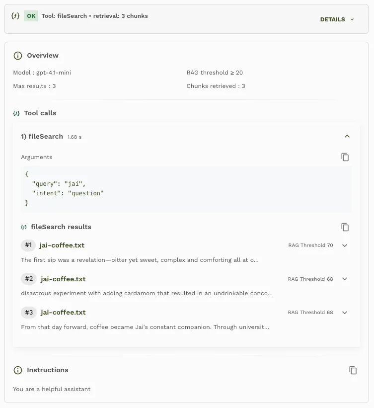
Step 1: Look at the search query

First, inspect the query sent to the knowledge search tool. The user's original message and the retrieval query do not necessarily have to be identical.

For example, the user might ask:

I bought the yearly plan yesterday. How long do I have to change my mind?

The model might search the knowledge base using something closer to:

annual subscription cancellation refund period

In the above image, "query": "jai", shows that the model searched for "jai". You can ignore the "intent" in the above picture.

In a semantic-search pipeline, that query is converted into an embedding and compared with stored chunk embeddings. So the system did not really search the entire question, but converted the question to a query, created an embedding from that query and searched for similar embeddings already stored.

Step 2: Look at the retrieved chunks

Next, inspect the chunks returned by the search. Read them. Do they contain the answer? Are some useful while others are merely related?

You can now see the path from question to answer:

Question
   ↓
Search query
   ↓
Retrieved chunks
   ↓
LLM answer

Three important RAG settings

While experimenting, three parameters are especially useful for understanding retrieval:

1. Chunk size
2. Maximum number of chunks
3. Minimum retrieval score (RAG Threshold in above image)

1. Chunk size

Chunk size controls how much text goes into each piece created from your document. Imagine this paragraph:

Predictable Dialogs offers several subscription plans.
Customers may cancel within 30 days.
Refunds are processed within five business days.
Enterprise customers may have separate contractual terms.

With smaller chunks, it might become:

Chunk 1: Predictable Dialogs offers several subscription plans.
Chunk 2: Customers may cancel within 30 days.
Chunk 3: Refunds are processed within five business days.
Chunk 4: Enterprise customers may have separate contractual terms.

With larger chunks, the whole passage might remain together. Neither approach is always better. Very small chunks may lose useful surrounding context; very large chunks may include too much unrelated information.

In Predictable Dialogs, you can choose the chunk size when configuring and uploading your knowledge. Try the same document with different chunk sizes and observe how retrieval changes.

2. Maximum number of chunks

Another setting is how many results the retriever is allowed to return. This is often called top-k retrieval:

Top 1  → retrieve at most one result
Top 5  → retrieve at most five results
Top 10 → retrieve at most ten results

Increasing this number gives the language model more potentially useful context. But more is not automatically better. Too many loosely related passages can increase token usage, latency, irrelevant context, and the chance of distracting the model.

Ask the same question with top 1, 3, 5, and 10, then inspect what changes.

3. Minimum retrieval score (RAG Threshold in the image above)

The third parameter is the retrieval threshold. Returned chunks can have a relevance or similarity score. In systems where scores are normalized to a range such as 0–1, a higher number generally means the result was considered more similar or relevant.

Chunk A — 0.89
Chunk B — 0.78
Chunk C — 0.52
Chunk D — 0.31

If the minimum score is 0.70, A and B might be returned while C and D are rejected. Lowering it to 0.30 would retrieve more broadly.

Retrieval scores are implementation-dependent. A score of 0.7 from one embedding model or vector database should not automatically be interpreted as equivalent to 0.7 from another. There is no universal “good RAG score.” Experiment with your documents and embedding model.

In Predictable Dialogs you can configure the minimum retrieval score and see how that changes which chunks are retrieved.

Top-k and minimum score work together

Suppose you configure:

Maximum chunks: 20
Minimum score: 0.80

If only three chunks score above 0.80, the retriever cannot return 20 qualifying results. It will return only those three.

Conceptually:

Find results
   ↓
Discard anything below the threshold
   ↓
Return at most K results

Top-k controls the maximum quantity. The score threshold controls the minimum acceptable relevance.

A simple experiment

Upload a document you understand well. Choose five questions:

• One whose answer is very obvious.
• One whose wording closely matches the document.
• One that asks the same thing using completely different words.
• One whose answer exists across several sections.
• One whose answer does not exist in the document.

Then experiment with chunk sizes of 200, 400, and 800, maximum results of 1, 3, 5, and 10, and different minimum retrieval scores.

For every experiment, inspect:

• The search query.
• The chunks retrieved.
• The score of each chunk.
• The final generated answer.

You will begin to see why particular questions succeed or fail.

What happens when RAG gives a bad answer?

If the generated answer is wrong, there are at least two different possibilities.

Retrieval failed

The correct information never reached the LLM. Maybe the document was chunked badly, the search query was poor, embedding search missed the right passage, the threshold was too high, or too few chunks were retrieved. Changing the generation prompt may not solve the underlying problem.

Generation failed

The correct passage was retrieved, but the LLM misunderstood it or generated an unsupported answer. That is a generation problem.

Inspecting the retrieved chunks lets you distinguish “Did we retrieve the wrong information?” from “Did the model reason incorrectly over the right information?” This is one of the most useful things to learn about RAG.

Once you understand the pipeline, build the pieces yourself

After experimenting with RAG visually, the architecture should start looking simpler.

At ingestion time:

Document
   ↓
Extract text
   ↓
Split into chunks
   ↓
Create embeddings
   ↓
Store embeddings

At query time:

Question
   ↓
Create query embedding
   ↓
Search vectors
   ↓
Retrieve relevant chunks
   ↓
Construct prompt
   ↓
Send prompt to LLM
   ↓
Generate answer

Start with the vector search pipeline

A useful first project is to implement retrieval yourself:

1. Chunk documents. Divide text into appropriately sized pieces. Later, explore fixed-size, overlapping, sentence-based, paragraph-based, heading-aware, and semantic chunking.
2. Generate embeddings. Send each chunk to an embedding model and receive its vector representation.
3. Store the vectors. Keep the vector, chunk text, document ID, page number, and other metadata together.
4. Embed the query. Create its embedding using the same embedding model.
5. Perform similarity search. Compare the query vector with stored vectors and return the nearest matches.
6. Give the results to an LLM. Construct a prompt containing the question and retrieved context.

At that point, you have built a basic RAG system.

Vector databases make more sense once you understand this

You will encounter technologies such as pgvector, Pinecone, Qdrant, Weaviate, Milvus, FAISS, and Chroma. Once you understand the pipeline, their role becomes clearer:

Store vector + content + metadata

Then:

Given query vector → find nearest stored vectors

Some platforms add ingestion, filtering, hybrid search, indexing, scaling, and document management. The underlying mental model remains the same.

And then RAG gets more sophisticated

Production RAG systems often contain additional steps:

Question
   ↓
Query rewriting
   ↓
Semantic search + BM25
   ↓
Retrieve 30 candidates
   ↓
Rerank candidates
   ↓
Keep best 5
   ↓
Build context
   ↓
Generate answer
   ↓
Verify answer

You might encounter hybrid search, metadata filtering, reranking, query expansion, multi-query retrieval, parent-child retrieval, contextual retrieval, agentic retrieval, citation extraction, groundedness checking, and retrieval evaluation. All of them are easier to understand once the basic loop is clear.

The important mental model

If you remember only one diagram from this article, make it this one:

                 INGESTION

Document → Chunks → Embeddings → Vector store

                 RETRIEVAL

Question → Query embedding → Similarity search → Relevant chunks

                 GENERATION

Question + relevant chunks → LLM → Answer

That is the foundation. Everything else in RAG attempts to improve one of those stages.

Learn RAG by looking inside it

RAG can appear complicated when we start by reading about vector databases, embedding models, rerankers, hybrid search, HNSW indexes, BM25, cosine similarity, and metadata filters.

A simpler learning path is to understand the pipeline, observe it working, change its parameters, understand why it fails, and then implement the pieces yourself.

With Predictable Dialogs, you can upload a document, ask questions, inspect the retrieval query, examine returned chunks and scores, and experiment with chunk size, retrieval count, and minimum score.

Once you can look at a RAG request and say, “This was the query, these were the chunks retrieved, and these are the passages given to the language model,” you understand the most important part of RAG.